Note: This is a guest post and not written by Yihui. Its author desires to remain anonymous. If anyone would like to contact the author, please contact me (Yihui). And if any statistical sleuths out there determine the author’s identity, please refrain from revealing it. Thank you.
INTEROFFICE MEMORANDUM
DATE: August 12, 1991
TO: □□□□□□□□□□□□□
FROM: □□□□□□□□□
SUBJECT: REVIEW OF S-PLUS STATISTICAL SOFTWARE
S-PLUS, from StatSci Corp., is a new type of statistical programming language. It was originally called “S” and developed by AT&T Bell Labs for UNIX. StatSci has expanded upon its capabilities and converted it for PCs. It differs from other statistical programming languages in many ways.
I consider it to be a cross between Minitab and object-oriented C. It is like Minitab in that it is interactive and fully integrates graphics and matrix operations with the statistical routines. Unlike Minitab, it also provides programming capabilities like object-oriented C. This makes the language very powerful, because one can easily and quickly develop nonstandard or repetitive routines.
This package has several advantages over more common statistical language packages such as SAS. SAS has DATA steps to prepare your data and PROC steps to analyze your data. In S-PLUS, there is no distinction. You can manipulate your data at any time, even within routines. This saves programming time and frees you from many of SAS’s constraints. Another major difference is that SAS comes in modules: one for basic functions, one for statistical analysis routines, one for graphics routines, one for matrix algebra, plus others. It even has a separate macro language for repetitive operations. This means you must buy – actually, rent – and install several products, and, more importantly, figure out how to program them together. This is not an easy task. With S-PLUS, these capabilities are integrated, which results in Exploratory Data Analysis (EDA) being very easy to perform, unlike SAS.
S-PLUS does have its disadvantages, mainly due to its data structure organization. The inherent matrix algebra-like organization requires a higher level of thinking than other packages do. Also, creating a data structure is a nontrivial task. However, once these concepts are mastered and a proper data set is created, analyzing the data is much easier and faster than other packages, because there are very few constraints to program around.
Another aspect that some people might consider a drawback is that S-PLUS does not have an exhaustive supply of routines to do everything under the sun. It doesn’t try to please everyone all the time. What it does try to do is provide a tool for scientist to analyze their data in a meaningful way. And if there is something else you want it to do, you can program it.
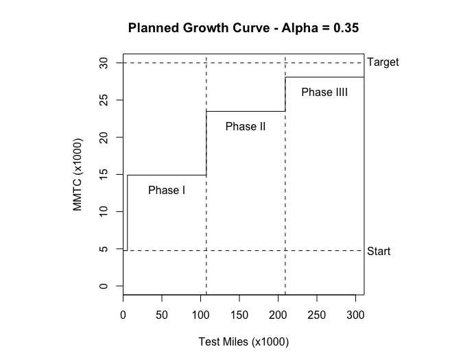
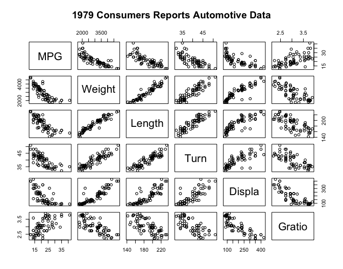
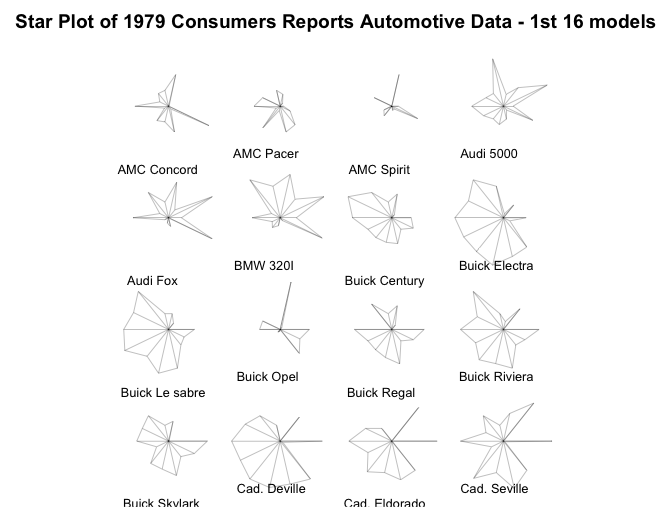
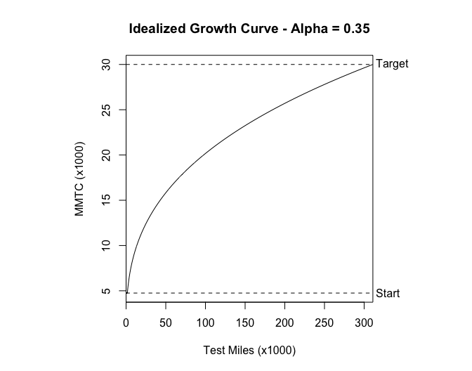
To give you a better idea of what S-PLUS can do, I’m enclosing an index of S-PLUS’s functions and examples of some of its capabilities. The first example is a matrix or “draftsman’s” plot of some automotive data. It is a multivariate technique to show the relationships between several variables. The second example is a partial listing of star plots of the same data set. The spikes on the stars represent a metric and the length of the spikes represents the value of the metric. This type of display makes it easy to see how items are similar or different. Both complex examples required only a few commands once the data structure was set up. The last examples are the plots and S-PLUS code for a reliability growth plan I did for □□□ □□□□□□□□ □□□□□□□ program. As you can see from the code, not much work was required to generate the plots, and if the parameters change, I can easily generate new plots by changing the arguments for the function.
I recommend that we buy two copies: one for the □□□□□□□ office and one for the □□□□□□□ office. The cost of one copy is $1195. But if you buy between two to five copies, the cost is $995 per copy. If you have any specific questions, either call me or call StatSci at (206) 283-8802.1
library(corrgram) pairs( auto[c(“MPG”, “Weight”, “Length”, “Turn”, “Displa”, “Gratio”)], main = “1979 Consumers Reports Automotive Data” )
stars( auto[1:16, ], main = “Star Plot of 1979 Consumers Reports Automotive Data – 1st 16 models”, labels = as.character(auto[1:16, “Model”]) )
ideal <- function(alpha, Ti, Mi, Mf) { # S function to plot idealized growth curve from alpha, Ti, Mi, & Mf. Ti <- Ti/1000 Mi <- Mi/1000 Mf <- Mf/1000 MMTC <- c(0:(10 * Mf))/10 mile <- exp(log(Ti) + (log(MMTC/Mi) + log(1 – alpha))/alpha) Tf <- max(mile) MMTC[MMTC < Mi] <- Mi header <- paste(“Idealized Growth Curve – Alpha =”, alpha) par(pty = “s”) plot(mile, MMTC, type = “l”, main = header, xlab = “Test Miles (x1000)”, ylab = “MMTC (x1000)”, xaxs = “i”) abline(h = Mf, lty = 2) abline(h = Mi, lty = 2) text(Tf, Mi, ” Start”, adj = 0, xpd = NA) text(Tf, Mf, ” Target”, adj = 0, xpd = NA) } ideal(0.35, 5500, 4750, 30000)
plan <- function(alpha, Ti, Mi, Mf) { # S function to plot planned growth curve from alpha, Ti, Mi, & Mf. # Assumes 3 Test Phases after initial test phase. T1 <- Ti/1000 M1 <- Mi/1000 M4 <- Mf/1000 T4 <- exp(log(T1) + (log(M4/M1) + log(1 – alpha))/alpha) # Calculate beginning and end of Test Phases. T2 <- (2 * T1)/3 + T4/3 T3 <- T1/3 + (2 * T4)/3 test.phase <- c(T1, T2, T3, T4) test.phase.1 <- test.phase[c(1, 2, 3)] test.phase.2 <- test.phase[c(2, 3, 4)] test.diff <- test.phase.2 – test.phase.1 # Calculate MMTC in between Test Phases. N <- (T1/M1) * (test.phase/T1)^(1 – alpha) N.1 <- N[c(1, 2, 3)] N.2 <- N[c(2, 3, 4)] N.diff <- N.2 – N.1 MMTC <- test.diff/N.diff # Make data vectors to plot. test.data <- c(0, T1, T1, T2, T2, T3, T3, T4) MMTC.data <- c(M1, M1, MMTC[1], MMTC[1], MMTC[2], MMTC[2], MMTC[3], MMTC[3]) # Plot data. header <- paste(“Planned Growth Curve – Alpha =”, alpha) par(pty = “s”) plot( test.data, MMTC.data, type = “l”, main = header, xlab = “Test Miles (x1000)”, ylab = “MMTC (x1000)”, xaxs = “i”, ylim = c(0, M4) ) abline(h = M1, lty = 2) abline(h = M4, lty = 2) abline(v = T2, lty = 2) abline(v = T3, lty = 2) text(T4, M1, ” Start”, adj = 0, xpd = NA) text(T4, M4, ” Target”, adj = 0, xpd = NA) text((T1 + T2)/2, MMTC[1] – 2, “Phase I”) text((T2 + T3)/2, MMTC[2] – 2, “Phase II”) text((T3 + T4)/2, MMTC[3] – 2, “Phase IIII”) } plan(0.35, 5500, 4750, 30000)